In order to find out the performance of an electric traction service at different schedule speeds, speed-time curves are replaced by trapezoidal and quadrilateral curves. From these simplified curves (trapezoidal and quadrilateral curves), the relationship between acceleration, retardation, average speed, and distance can be obtained.
The use of these simplified curves saves the labor of repeating the calculations a large number of times and also while performing calculations there is no need for much information related to motor characteristics.
While constructing trapezoidal and quadrilateral speed time curves, the following points need to keep in mind,- The area enclosed by the curve, acceleration, and braking retardation values must be similar to that of the original speed-time curve.
- The running and coasting periods are replaced by a constant speed period for a long-distance run as shown by the trapezoidal speed time below.
- The initial acceleration and coasting periods are extended for the short distance of run as shown by the quadrilateral speed-time curve.
- The area under the trapezoidal and quadrilateral curves and the actual speed time curve should be same.
In the two simplified curves, the trapezoidal speed-time curve corresponds to the speed-time curve of mainline service and the quadrilateral speed-time curve corresponds to the speed-time curve of urban and suburban services where short distances are involved. Let us see the construction and calculations of trapezoidal and quadrilateral speed-time curves.
Trapezoidal Speed Time Curve :
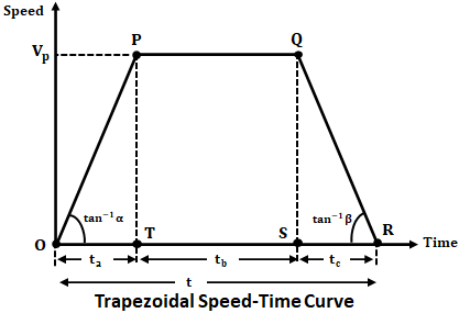
The trapezoidal speed-time curve is a close approximation to the speed-time curve of mainline service where the free-running period of the locomotive is long. The below shows the trapezoidal speed-time curve OPQR where speed is taken on the y-axis and time on the x-axis.
Let,- S = Distance between two stations or stops in meters.
- t = Actual run time between two stops in sec.
- α = Acceleration during starting point in m/s2.
- β = Retardation during braking in m/s2.
- Vp = Peak value of speed in m/sec.
- Vavg = Average value of speed in m/sec.
- ta = Time of acceleration in sec.
- tb = Time of free-running period in sec.
- tc = Time of braking in sec.
The total distance between stops is given by the area of trapezium OPQR.
S = Area of OPQR
S = Area of OPT + Area of PQST + Area of QRS
S = A1 + A2 + A3 ...(1)
We know that acceleration is defined as the rate of change in velocity. From the figure, we have,
α = Vp/ta and β = Vp/tc ...(2)
In the above curve, the area of triangle OPT is,
A1 = 1/2 × Base × Height = 1/2 × ta × Vp ...(3)
Area of PQST,
A2 = length × Breadth = Vp × tb ...(4)
Area of triangle OPT,
A3 = 1/2 × Base × Height = 1/2 × tc × Vp ...(5)
Therefore, substituting equations 3, 4, 5 in equation 1, we get,
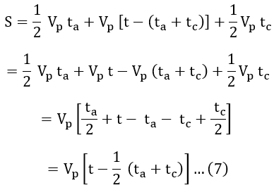
S = 1/2 × ta × Vp + Vp × tb + 1/2 × tc × Vp ...(6) But from figure, we have,
tb = [t - (ta + tc)]
Substituting above tb value in equation 6 we get,
From equation 2 we have,
α = Vp/ta ⇉ ta = Vp/α ...(8)
β = Vp/tc ⇉ tc = Vp/β ...(9)
On adding equation 8 and 9 we get,
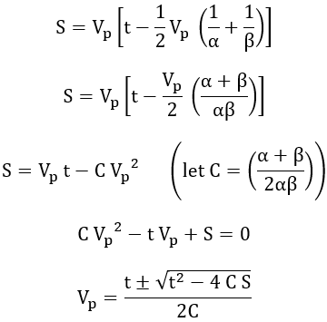
ta + tc = Vp × 1/α + 1/β
Substituting the above ta + tc value in equation 7, we get,
In the above equation, the +ve sign cannot be adopted, as the value of Vp obtained by using the +ve sign will be much higher than what is possible in practice. Hence -ve sign will be used and therefore, we have,
From the above equation, an unknown quantity can be determined by substituting the values of known quantities.
Quadrilateral Speed Time Curve :
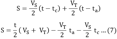
The quadrilateral speed-time curve is a close approximation to the speed-time curve of urban or suburban services where the distance between stops is small. The below shows the quadrilateral speed-time curve OSTU where speed is taken on the y-axis and time on the x-axis.


